CMSI 2210: Welcome to Week 07
This Week's Agenda
For this week, here's the plan, Nan…

|
|
Really Truly CPU Processors
The Stanley/Penguin
machine and it's assembly language give us a heads-up on how actual
CPU machines work. Now that we understand the idea of loading, storing, reading/writing to a
port, the difference between arithmetic instructions [add/sub/mod etc.] and logic instructions
[and/xor etc.], and how to mimic if
statement operations [SUB followed by JZ, JGZ, JLZ],
we can move on to the real thing.
There are two major processor types that you'll find in use today. One is based on the Intel architecture which has been around since dinosaurs but which has been constantly updated. Intel makes these, of course, but so does Advanced Micro Devices [AMD]. The two chip makers have CPU chips that are based on essentially the same architecture. The IA-32 is the instruction set architecture [ISA] of Intel's most successful line of 32-bit processors, and the Intel 64 ISA is its extension into 64-bit processors. [Actually Intel 64 was invented by AMD, who called it x86-64]. These are CISC processors as we've seen previously.
The other type of processor in [even more] widespread use is the ARM processor which is found in nearly all portable devices such as cell phones, tablets, new Mac computers, and many more. These are RISC processors which have many similarities to the x86-64 chips, but also have some very important differences as we will see.
Here are some links to more information and comparisons of the two families' products:
- Comparison from PC Magazine 2021
- Shopinbrand comparison
- Digital Trends comparison
- The ARM main page
- ARM Architecture Documentation Page
- A7 MPCore Technical Reference Manual
- ARMv7 Architecture Manual
The X86 architecture
These two [Intel and AMD] architectures are so common, they are described in a single set of manuals. Even though the set is MASSIVE, there are several sections that are worth a) reading; and b) knowing about as a reference.
The following notes briefly summarize the former architecture only.
x86-64 Architecture Diagram
The basic architecture of the x86-64 is described in Volume 1 of the System Developer's Manual. The following diagram is taken directly from Chapter 3 in this volume:
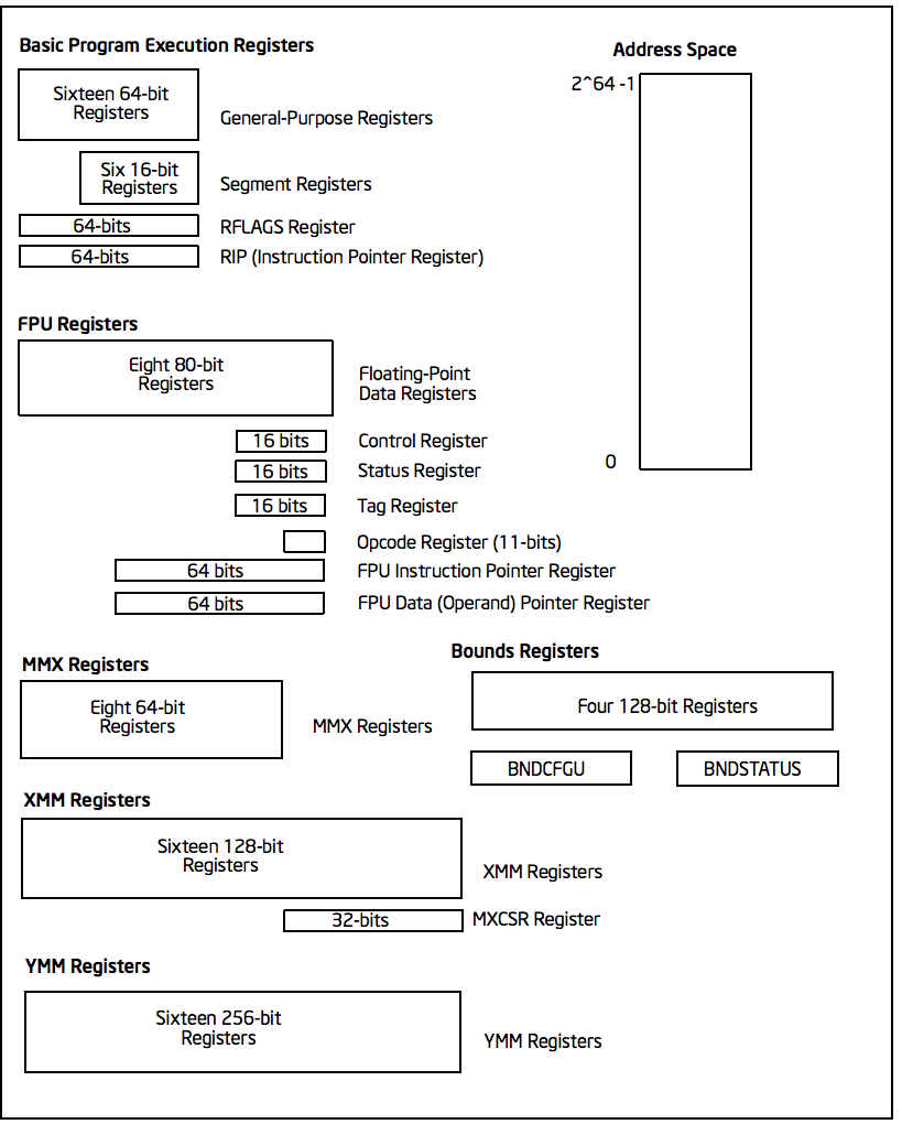
Registers
Application Programmers generally use only the general purpose registers, floating point registers, XMM, and YMM registers.
General Purpose Registers
These are 64 bits wide and used for integer arithmetic and logic, and to hold both data and pointers to memory. The registers are called R0...R15. Also:
- You can access the lower order 32-bits of each register using the names R0D...R15D. The
D
stands fordoubleword
because strangely, the wordword
on this platform refers to a 16-bit quantity. Why? Backward compatibilty! The x86-64 grew out of a 16-bit processor family created in the 1970s. [Wait... the '70s??? IKR?] - You can access the lower order 16-bits of each register using the names R0W...R15W.
- You can access the lower order 8-bits of each register using the names R0B...R15B, also R0H or R0L.
- R0...R7 have aliases RAX, RCX, RBX, RDX, RSP, RBP, RSI, RDI, respectively.
- R0D...R7D have aliases EAX, ECX, EBX, EDX, ESP, EBP, ESI, EDI, respectively.
- R0W...R7W have aliases AX, CX, BX, DX, SP, BP, SI, DI, respectively.
- R0B...R7B have aliases AL, CL, BL, DL, SPL, BPL, SIL, DIL, respectively.
RIP and RFLAGS
RIP is the instruction pointer and RFLAGS is the flags register.
Segment Registers
These are CS, DS, SS, ES, FS, and GS. I haven't used them in 64-bit programming, only in 16-bit and 32-bit programming.
XMM Registers
These are 128-bits wide. They are named XMM0...XMM15. You use them for both floating-point and for integer arithmetic operations. You can do operations on 128-bit integers, but you can also take advantage of their ability to do operations in parallel as follows:
- Two 64-bit integer operations in parallel
- Four 32-bit integer operations in parallel
- Eight 16-bit integer operations in parallel
- Sixteen 8-bit integer operations in parallel
- Two 64-bit floating-point operations in parallel
- Four 32-bit floating-point operations in parallel
YMM Registers
These are 256-bits wide. They are named YMM0...YMM15. You use these for floating-point arithmetic. You can do:
- Four 64-bit floating-point operations in parallel
- Eight 32-bit floating-point operations in parallel
and some other crazy things.
FPU Registers
There are eight registers used for computing with 80-bit floating point values. That's right, 80-bits. The registers don't have names because they are used in a stack-like fashion.
Other Registers
Application programmers can remain oblivious of the rest of the registers:
- The 8 32-bit processor control registers: CR0, CR1, CR2, CR3, CR4, CR5, CR6, CR7. The lower 16-bit space of CR0 is called the Machine Status Word [MSW].
- The 4 16-bit table registers: GDTR, IDTR, LDTR and TR.
- The 8 32-bit debug registers: DR0, DR1, DR2, DR3, DR4, DR5, DR6 and DR7.
- The 5 test registers: TR3, TR4, TR5, TR6 and TR7.
- The memory type range registers
- The machine specific registers
- The machine check registers
Register Operations
Just like in Stanley/Penguin, we have a set of load and store operations that put things into
the registers. We use these just like we used the accumulator before, only there are LOTS AND
LOTS of them now. The instructions still take the same form, only since we have multiple
registers, we have to specify the source AND the destination. For example, to load the value
0xAAAAAAAA into the RAX register, you would use
MOV rax, 0xAAAAAAAA
Instruction Set
See the SDM Volume 1, Chapter 5 for a nice overview of all of the processor instructions and Volume 2 for complete information.
This
link goes to a PDF of Volume 2 of the Intel Software Developer's Manual, which is the bible.
You can download a copy for free. Be aware, it's pretty big. Some browsers will open it for
you online, some won't always. Once you get a copy, take a look at Chapter 3. That has all
the general information about mnemonics for the instructions, as well as instructions beginning
with A – L. Then take a look at chapter 4, which gives information for
instructions beginning with M – U. Finally, the rest of the instructions
are provided in chapter 5 for those beginning with V – Z.
In the mnemonics, the vertical bar means OR, the square brackets mean OPTIONAL, and parentheses are used for grouping. For example:
SH(L|R)[D]stands forSHL,SHR,SHLD, and/orSHRD. Notice you can have eitherSHLorSHRBUT NOT justSH. The square brackets around theD
mean that it is optional, so you can add it to the end to make two more instructions.PUSH[A[D]]stands forPUSH,PUSHA, and/orPUSHAD.
Typical or Most-used Instructions
There are literally hundreds of instructions in the instruction set for this processor, but
much of what we will explore can be done with a few simple ones. One of the most common is
the MOV instruction, as we've seen, which puts a value from somewhere
into somewhere else. The locations all depend on the addressing
mode that is being used, of course, but you can think of it as
MOV <destination> <source>.
Some of the other common mnemonics are listed below:
Note: the letters in suqare brackets are optional and can be added or not based on what you are
trying to accomplish with the CISC instructions. This is part of what makes it a CISC
computer!
| Mnemonic | Description |
|---|---|
| MOV dest, source | Moves data from source to destination this is the default; see next lines |
| MOVB dest, source | Moves a byte of data from source to destination
|
| MOVW dest, source | Moves a word [16 bits] of data from source to destination
|
| MOVL dest, source | Moves a d word [32 bits] of data from source to destination
|
| MOVQ dest, source | Moves a quad word [64 bits] of data from source to destination
|
| LEA value (%ebp, %ecx, mult) | Load Effective Address as computed by equation EAX := value + (EBP + (mult * ECX)) |
| LEAL value (%ebp, %ecx, mult) | Load Effective Address as computed by equation EAX := value + (EBP + (mult * ECX)) |
| PUSH register | Pushes the value of register onto the stack |
| POP register | Pops the valur on top of the stack into the register |
| ADD[L] dest, source | Adds the value of source to destination Similar for SUBL, MUL, DIVL instructions and the Ldoes the same thing as with the MOV instruction
|
| CMP[L] dest, source | Compares two integers by subtracting the first from the second |
| NEG[L] location | Negates [makes two's complement] of value at location |
| AND[L] | Performs logical AND with two operands |
| OR[L] | Performs logical OR with two operands [also NOTL for 1's complement] |
| JMP dest | Jump unconditionally to the dest |
| Jcc dest | Jump conditionally to the dest conditions are most often e, z, g, l can also insert nfor notas in JNE can also append efor equalas in JGE |
There are quite a few LESS instructions in the ARM instruction set, but they are very powerful as you can see. Here are some of the most frequently used instructions:
| Mnemonic | Description |
|---|---|
| LDR dest, source | Loads a value from source to destination |
| LDR = immediate | Loads a hard-coded number [numeric literal] |
| STR src, [base] | store register |
| ADD dest, src1, src2 | dest = src1 + src2 |
| ADD dest, src1, #imm | dest = src1 + numeric literal |
| SUB dest, src1, src2 | dest = src1 - src2 |
| SUB dest, src1, #imm | dest = src1 - numeric literal |
| RSB dest, src1, src2 | dest = src2 - src1; often used for negation |
| RSB dest, src1, #imm | dest = src2 - numeric literal |
| MUL dest, src1, src2 | low order 32 bits |
| SDIV dest, src1, src2 | dest = src1/src2 |
| CMP src1, src2 | sets flags for src1-src2 |
| LSL dest, src, #shift | logical shift left, src shifted by # into dest, zero fill |
| LSL reg, #shift | logical shift left, register is shifted by numeric literal, zero fill |
| LSR dest, src, #shift | logical shift right, same as LSL, zero fill |
| LSR reg, #shift | logical shift right, same as LSL, zero fill |
| ASR dest, src, #shift | arithmetic shift right, preserves sign |
| ROR reg, shift | rotate right, like shift but rotates bits around |
| AND reg, mask | bitwise AND using register values, clobbers register |
| AND reg, #mask | bitwise AND using immediate values, clobbers register |
| AND dest, src, #mask | bitwise AND using immediate value, keeps register |
| ORR reg, mask | bitwise OR using register values, clobbers register |
| ORR reg, #mask | bitwise OR using register values, clobbers register |
| ORR dest, src, #mask | bitwise OR using immediate value, keeps register |
| EOR reg, mask | bitwise exclusive OR using register values, clobbers register |
| EOR reg, #mask | bitwise exclusive OR using register values, clobbers register |
| EOR dest, src, #mask | bitwise exclusive OR using register values, clobbers register |
| MOV dest, src! | move reg to reg |
| MVN dest, src | bitwise NOT |
| B label | unconditional branch |
| BL label | subroutine call |
| BX reg | branch indirect |
they also have 'condition codes' that can be attached: EQ, NE, GT, LT, GE, LE, PL, MI
Addressing Modes
In protected mode, applications can choose a flat or segmented memory model [see the SDM Volume 1, Chapter 3 for details]; in real mode only a 16-bit segmented model is available. Most programmers will only use protected mode and a flat-memory model, so that's all we'll discuss here.
A memory reference has four parts and is often written as:
[SELECTOR : BASE + INDEX * SCALE + OFFSET]
The selector is one of the six segment registers; the base is one of the eight general purpose registers; the index is any of the general purpose registers except ESP; the scale is 1, 2, 4, or 8; and the offset is any 32-bit number. (Example: [fs:ecx+esi*8+93221].) The minimal reference consists of only a base register or only an offset; a scale can only appear if there is an index present.
Sometimes the memory reference is written like this:
selector
offset(base,index,scale)
Data types and How They Are Handled
The data types that can be used are NOT like what we're used to. Instead of int, char, and double
we have the following, which are based on the number of bits:
| Type Name | Number of bits | Bit Indices |
|---|---|---|
| Byte [byte] | 8 | 7…0 |
| Word [word] | 16 | 15…0 |
| Doubleword [dword] | 32 | 31…0 |
| Quadword [qword] | 64 | 63…0 |
| Doublequadword [dqword] | 128 | 127…0 |
Little Endian-ness
Remember big-endian and little-endian? Well, now it becomes important. The IA-32 architecture is a little-endian machine, which means that it stores the least significant bytes at the lower byte of memory. Here is a table to show you some examples.
      0    12
      1    31       byte @ 9 = 1F
      2    CB       word @ B = FE06
      3    74       word @ 6 = 230B
      4    67       word @ 1 = CB31
      5    45       dword @ A = 7AFE0636
      6    0B       qword @ 6 = 7AFE06361FA4230B
      7    23       word @ 2 = 74CB
      8    A4       qword @ 3 = 361FA4230B456774
      9    1F       dword @ 9 = FE06361F
      A    36
      B    06
      C    FE
      D    7A
      E    12
Notice that if you are storing a word at a location, you'll specify the lowest order byte address, but the values will be stored at successively higher addresses. This can get very confusing when you are learning to program on this architecture, because you can end up accidentally writing over your values that you've stored if you are using the wrong sizes or aren't calculating the addresses correctly.
Bit shifting for fun and profit
One thing that is interesting about working directly with registers is that we can shift the bits in the registers around. There are a number of reasons why we would want to do that:
- multiplication or division by some power of two
- figuring out a CRC or hashing value may require it
- some compression algorithms shift bits as part of encoding
- bit manipulation is used in UTF-8 encoding
- parity generation
- many more!
Remember that bit shifting is different than bit rotation. When we shift bits, we move the pattern left or right and the empty spaces on the end are [usually] zero-filled. With rotation, what comes out of one side goes back into the other side.
Basic Input/Output System [BIOS] Calls [click to read/close]
BIOS calls are important since they are the lowest level system calls that can be made. In modern processor programming, these are RARELY used, even in assembly coding, because they are at SUCH a low level. There are the calls that are used to get your system booted and running.
We have seen, or will see, how some of these system calls
are made later. However, it
is MUCH easier for our purposes to use the C
routines such as printf() and
scanf() to handle the jobs of these system BOIS calls. In fact, those C
functions INTERNALLY call the system calls!
Click here to read more…
The ARM Architecture
The ARM processor is designed as a low-power, RISC-style processor which provides the flexibility to be applied to a number of applications. You may be familiar with this processor if you have done any programming with a Raspberry Pi Single Board Computer [SBC]. However, due to its low-power nature the processor is used a a great many modern devices, including the cell phone on which you might be reading this!
The ARM architecture actually has three main variants, called profiles:
- Armv7-A: The application profile for systems supporting the Arm and Thumb instruction sets, and requiring virtual address support in the memory management model.
- Armv7-R: The real-time profile for systems supporting the Arm and Thumb instruction sets, and requiring physical address only support in the memory management model.
- Armv7-M: The microcontroller profile for systems supporting only the Thumb instruction set, and where overall size and deterministic operation for an implementation are more important than absolute performance.
There is one other variety which is used in your Mac computers, the M1-M2-...-M5 CPU. These are ARM-style processors but are implemented by Apple and are thus known as APPLE SILICON.
Since it is a RISC processor, the ARM instruction set is much smaller than the X86 instruction set. Don't let that fool you though. As we've seen with Stanley Penguin, all you really need to get work done is 16 basic instructions and a single register! In fact, [as you will learn in your Theory of Computation class later, all you REALLY REALLY need is a machine that can read or write a single bit of information, and move a tape one way or the other by a single slot — a device that is known as a Turing Machine.
The fact that the instruction set is small means we don't have sophisticated instructions such as
ASCII Adjust for Addition
or Dot Product of Packed Singles
. Instead, we get twice the
number of general purpose registers and the ability to typically do many more instructions in the same
amount of time. Most of the instructions in an ARM machine can be done in one or two clock cycles,
while the X86 machine may take many clock cycles for a typical instruction.

| One of the first things to note about the ARM instruction set architecture is that
all of the instructions are fixed length,
meaning they all have the same number of bits in every instruction. Contrast this with
the X86-64 which, because of its multiple addressing modes, can have instructions with
VERY different numbers of bits. This is part of the reason that an X86-64 processor runs
slower than an ARM process — the A second thing that is a bit different with ARM is that it is a load/store architecture. This means the processor uses dedicated instructions to load data from memory into the processor's internal registers. A CPU function then performs any processing operations using only the values in these registers as operands, with the results then saved to memory using corresponding dedicated store instructions. |
The simplicity of this architecture is why it was used as a model for the Stanley/Penguin machine!
In that case, there is only one 32-bit register, called the Accumulator
and all of the
instructions use that single register. For ARM, though, there are 32 registers of 32 bits each!
ARM Fundamental Data Types
Here are brief descriptions of the internal architecture parts of the ARM processor. Note that we are using the ARM-7 as our model:
- The priority encoder works as digital data conversion circuit which converts multiple input signals into a binary code representing the highest priority active input. The priority encoder ensures that interrupts are processed in the correct order, which is critical for maintaining the responsiveness and stability of the overall system.
- The multiplexer, also known as a MUX, is a digital circuit that selects one of several input signals and forwards it to a single output. The primary purposes of a multiplexer in ARM architecture is to enable the processor to access multiple inputs through a single port. This is particularly useful when dealing with data that is stored in different locations or formats, as it simplifies the communication process between the processor and the memory.
- The Arithmetic Logic Unit [ALU] performs arithmetic operations such as addition, subtraction, multiplication, and division on binary data. In addition to arithmetic operations, the ALU in ARM architecture is also responsible for performing logical operations such as AND, OR, NOT, and XOR. The ALU in ARM architecture is typically designed to support a range of data types, including integers, floating-point numbers, and Boolean values. It also includes a range of conditional operations, such as comparisons and conditional branching.
- The Booth multiplier in ARM architecture is to perform efficient and accurate multiplication of binary numbers. The Booth multiplier uses a combination of shifting and addition/subtraction operations to perform the multiplication, which reduces the number of required operations and thus increases the speed of the computation.
- The barrel shifter in ARM architecture is to perform efficient and flexible bit-manipulation operations on binary data. The barrel shifter can shift or rotate a binary value by any number of bits, allowing for efficient implementation of operations such as multiplication, division, and logical operations. The barrel shifter in ARM architecture is also useful for implementing data packing and unpacking operations, which are commonly used in multimedia and image processing applications.
- The Control Unit in ARM architecture is to manage the operation of the processor by coordinating the activities of other components, such as the ALU, memory, and input/output devices. The Control Unit is responsible for reading instructions from memory, determining the appropriate operation to perform based on the instruction, and executing the operation by sending control signals to the other components of the processor.
- The Program Status Register [PSR] provides a mechanism for tracking the state of the processor during the execution of instructions.
- The General Purpose Registers [GPRs] are a set of registers in the ARM architecture that are used to store temporary data and memory addresses during the execution of instructions. These registers are used by the processor to store data that is being processed, as well as memory addresses that are used to access data in memory.
- The Special Function Registers [SFRs] are another set of registers that have specific functions and are used to configure or control various system operations. The purpose of the SFRs in ARM architecture is to provide a flexible and efficient mechanism for configuring and controlling various hardware functions, such as interrupt handling, memory management, and system-level control operations.
ARM Fundamental Data Types
Much like with the X86 architecture, ARM supports data types that are based on the number of bits for each piece of data. However, there are differences, as you can see in the following table:
| Data Type | Size [bits] | Typical Use |
|---|---|---|
| Byte | 8 | Characters, byte-size ints |
| Halfword | 16 | 16-bit integers and floats |
| Word | 32 | 'wide' characters, integers and floats |
| D-Word | 64 | Doubleword integers Double precision floating point Packed integers Packed half-precision floating point Packed single-precision floating point |
| Quadword | 64 | Quadword integers Packed integers Packed half-precision floating point Packed single-precision floating point Packed double-precision floating point |
Bits in these data types are numbered just as you would expect, starting at the right side and moving to the left, with the right-most bit being bit zero, the LSB, corresponding to the zero-eth power of two [the 'ones' place].
ARM also supports both big-endian and little-endian representations.
ARM Numerical Data Types
All ARM numerical types are stored using one of the fundamental data types listed above. The following
table shows the corresponding C
data types that match up:
| Data Type | Size [bits] | CType | Type Definition |
|---|---|---|---|
| Signed int | 8 | char | int8_t |
| 16 | short | int16_t | |
| 32 | int, long | int32_t | |
| 64 | long long | int64_t | |
| Unsigned int | 8 | unsigned char | int8_t |
| 16 | unsigned short | int16_t | |
| 32 | unsigned int, unsigned long | int32_t | |
| 64 | unsigned long long | int64_t | |
| Float/Double | 16 | N/A | N/A |
| 32 | float | N/A | |
| 64 | double | N/A |
Next week we will see more about the X86 and ARM instruction sets and how they work.
The NVidea GPU Architecture
The NVidea architecture is actually a CPU plus a GPU architecture, which is built specifically for accelerated performance at the terabyte scale. It uses the ARM architecture to make a a CPU and server architecture which is constructed for accelerated computation. It includes an ultra-fast NVIDIA chip-to-chip interconnect, delivering 900 GB/s of total bandwidth. DANG!
The NVidea GPU is built around the idea of a Streaming Processor or SM. This basic building block is sort of like a mini-ARM CPU, but is extremely optimized to execute instructions VERY VERY fast. Here is a look inside:

Tensor Cores are specialized high-performance compute cores for matrix multiply
and accumulate (MMA) math operations. These cores are coupled with many specialized registers to
improve throughput, and are then ganged
together to make things even faster. This type of
architecture spawns the name Compute Unified Device Architecture, or
CUDA, which includes a high-level device architecture, a parallel
programming model, and a software platform that augments the C
language, similar to the
way the C++
language adds to the basic definition of C
.
In such a device, the GPU hardware units are all exactly the same, and are all capable of a wide
range of computational activities. These devices are known as Streaming
Multiprocessors or SM's
. The Tensor Cores are the main components of the SMs,
as you can see from the diagram.
GPU's can execute more threads in parallel than a normal CPU can. A
thread or thread of execution is the lowest unit of
programming for a GPU. A thread has its own registers which it uses for operation, but very
little else. Like a thread on a CPU, a GPU thread can have a private instruction pointer/program
counter. However, GPU programs are generally written so that all the threads in a collection
[called a warp] share the same instruction pointer, executing instructions in
lock-step with each other. Mostly threads are exeucuting the same instructions as each
other which provides massive parallelism on shared data spaces. A single CUDA core will
execute instructions from a single thread.
Warps provide a distinct advantage over normal CPU's. Normal CPU's must use a few hundred to a few thousand clock cycles [more like a microsecond than a nanosecond] due to the need to save the current state [or context of one thread and restore the context of another. In GPU threads, each thread has its own private registers allocated from the register file of the SM, so context switches on the GPU do not require any data movement to save or restore a thread's context. Because of these optimizations, a single SM on a GPU can concurrently execute up to 2048 threads split across 64 thread groups of 32 threads each. With 132 SMs, that's a total of over 250,000 concurrent threads executing simultaneously! Here is a diagram that shows you the difference between a |

|
Note that each of the little green core blocks in the GPU side of the diagram is actually a SM. Refer to the prior drawing to see how that all lines up. Also remember that CUDA cores are GPU cores that execute scalar arithmetic instructions like 2 + 2, while Tensor cores are GPU cores that operate on entire matrices with each instruction!
CUDA enables general-purpose computing on GPUs. It operates as a heterogeneous computing system, leveraging both the CPU [host] and GPU [device] to accelerate data-parallel workloads. The CPU manages the application and memory, launching kernels [functions] on the GPU. Data must be explicitly transferred between host memory and device memory. Computation is organized into a grid of thread blocks, which are further divided into individual threads. All threads in a block execute on a single SM and can communicate via shared memory. Kernels launch thousands of threads simultaneously. Threads within a block can synchronize, but threads in different blocks must remain independent to allow flexible scheduling across SMs. CUDA exposes a layered memory system including registers, shared memory, L1/L2 caches, and global memory, allowing developers to optimize for performance.
Interestingly enough…
It is highly unlikely that you will ever directly program a GPU directly in assembly language. Although it exists, the assembly language is so low-level that the language to use for any programming on a GPU is done at a higher level, using the CUDA language.
If you want to go even higher up the chaing, there are Python libraries like PyTorch that you can install for free to give you even more flexibility at a higher level of abstraction.
Still, this architectural information is good to know so you can be effective in using the GPU in your computer when you need it!
In-class Exercise
Learning outcomes: The student will learn more about using the 'nasm' language, including: 1) translating the simple concepts learned so far into real assembly; 2) accessing registers; 3) using nasm mnemonics for a simple program; 4) augmenting existing 'nasm' code per specifications; 5) using looping in the 'nasm' language.
We're going to take a shot at moving from Stanley/Penguin to 'nasm' by
porting[translating from one programming language to another] the code for thepowers of twoprogram to 'nasm'. Here is the code from the first homework assignment which printsHello, Worldto the display. Your task is to modify this code to put in a loop so that it outputs the powers of two like the Stanley/Penguin code should do. Note that this code uses theCprintf()function to make the task easier to get working to start with.
Here is the starting code:
Mac OS x86-64 version [uses printf() "C" library call]
         global   _main                ; this is the main entry point
         extern   _printf              ; external code from "C" library
         default  rel                  ; default to 'relative' addressing

         section  .text                ; text [code] segment

_main:
         push     rbx                  ; save this for return to O/S
         lea      rdi, [message]       ; load effective address of message
         call     _printf              ; call "C" printf function

exit:    pop      rbx                  ; restore base pointer
         ret                           ; return to O/S

         section  .data
message: db       "Hello, world!", 0x0A, 0x00
Mac OS ARM version [uses printf() "C" library call]
         .global _main
         .align  2

_main:
         adrp  x0,   message@PAGE
         add   x0,   x0,   message@PAGEOFF
         bl    _printf

_exit:
         mov   x0,   #0
         mov   x16,  #1
         svc   0

.data
.balign  4
message: .ascii   "\n\n   Hello, world!\n\n"
Windows version
         global   _main                ; this is the main entry point
         extern   _printf              ; external code from "C" library

         section  .text                ; text [code] segment

_main:
          push    message              ; windows is different! push instead of lea
          call    _printf              ; call printf()
          add     esp, 4               ; we 'pushed' so we restore stack pointer

          ret                          ; return to O/S

message:  db  'Hello, World', 0x0A, 0x00
Assemble, link, and run with the following commands:
Mac OS X86 version [updated]
      nasm -fmacho64 sayhello.nasm
      ld -macosx_version_min 10.7 sayhello.o -o sayhello
      ./sayhello
Mac OS ARM version [updated]
      as -o sayhello.o sayhello.arm
      ld -macosx_version_min 10.7 -o sayhello sayhello.o -lSystem -syslibroot `xcrun -sdk macos --show-sdk-path` -e _main -arch arm64
      ./sayhello
Windows version
      nasm -fwin32 sayhello.nasm
      gcc sayhello.obj -o sayhello.exe
      sayhello
For an extra challenge, see if you can get these system call versions to work! The mac one should be straightforward, but the windows one may be more difficult to get working…
Mac OS x86-64 version [uses Mac system calls]
         global      start                   ; on Linux this should be "_start"

         section     .text
start:   mov         rax, 0x02000004         ; system call for write [Linux should be "_start"]
         mov         rdi, 1                  ; file handle 1 is stdout
         mov         rsi, message            ; address of string to output
         mov         rdx, 13                 ; number of bytes
         syscall                             ; invoke operating system to do the write
         mov         rax, 0x02000001         ; system call for exit [Linux use "60"]
         xor         rdi, rdi                ; exit code 0
         syscall                             ; invoke operating system to exit

         section     .data
message: db          "Hello, World", 10
Windows version
; Define variables in the data section
            section  .data
hello:      db       'Hello world!',10
helloLen:   equ      $-hello

; Code goes in the text section
            section  .text
            global   _main

_main:      mov      eax,  4            ; 'write' system call = 4
            mov      ebx,  1            ; file descriptor 1 = STDOUT
            mov      ecx,  hello        ; string to write
            mov      edx,  helloLen     ; length of string to write
            int      80h                ; call the BIOS interrupt

; Terminate program
            mov      eax,  1            ; 'exit' system call
            mov      ebx,  0            ; exit with error cod
            int      80h                ; call the BIOS interrupt
Assemble, link, and run with the following commands:
Mac OS version [updated]
nasm -fmacho64 sayhello.nasm ld -macosx_version_min 10.7 sayhello.o -o sayhello ./sayhello
[NOTE: this is a different command than the original, using thelinkerinstead ofgcc] You can also use semicolons or ampersands to separate commands and put them on the same line:
nasm -fmacho64 sayhello.asm && ld -macosx_version_min 10.7 sayhello.o -o sayhello && ./sayhello nasm -fmacho64 sayhello.asm;ld -macosx_version_min 10.7 sayhello.o -o sayhello;./sayhello note the semicolons ↑ ↑
Windows version
      nasm -fwin32 sayhello.nasm
      gcc sayhello.obj -o sayhello.exe
      sayhello

      You can also use ampersands to separate commands and put them on the same line:

      nasm -fwin32 sayhello.asm && gcc sayhello.obj -o sayhello.exe && sayhello

      [NOTE: you CANNOT use the semicolon to separate commands on the Windows command line.]
You'll need to look up a few things on line to do this. First, you need to see how to do comparisons,
which in nasm can be done with the cmp instruction. You'll also need to use the
inc and the mov instructions. You will also need the add
instruction in some form. There may be some others, too.
Your task is to look these up and implement the Stanley/penguin program using nasm. Here is the Stanley/Penguin code:
   ; demo.stpn
   ; program to output the powers of 2 up to 1,000,000
   ; output goes to port 100  [hex 0x64]
   ; copied from cmsi 284/2210 web pages

   0         JMP     start    ; begin by jumping over the data area
   1 pow:    1                ; store the current power value here
   2 limit:  1000000          ; we'll be computing powers up to this amount
   3 start:  LOAD    pow      ; bring the value into accumulator to use
   4         WRITE   100      ; output the current power
   5         ADD     pow      ; adding to itself makes the next power!
   6         STORE   pow      ; store it (for next time)
   7         SUB     limit    ; we need to compare with limit, subtracting helps
   8         JLZ     start    ; if not yet past limit, keep going
   9 end:    JMP     end      ; this "stops" the program!
Weekly Wrap-up
That's it for this week. Next week we'll get into system calls and more details of nasm.
Then in a few weeks, we'll see how to write 'nasm' code that can be called as a function from
C
, and then we'll also see how to do it the other way round. Hmmm... maybe we'll do
THAT the other way round, I haven't decided yet… 😁