CMSI 486: Welcome to Week 06

This Week's Class Agenda

• Transaction Processing Continues/Concludes
• Concurrency and Locking methods
• Indexing

Transaction Processing Conclusion

Recovery

When a transaction fails, it usually means that the database must be restored to the state which was the most recent consistent state before the failure occurred. To facilitate this operation, the DBMS must keep pertinent information about all the various transactions, using the transaction manager, as we've seen. This information is usually kept in a system log, a transaction log, or both. There are two different types of scenarios for which recovery must be performed:

• If the database [and other operational system features] is damaged in a catastrophic way, such as by a hard disk crash, malware, or some data corruption event, the method used for recovery must put back a copy of the data that was backed up to an archive of some type. This might be backup tapes, a set of hard drives at a remote location, or some other scheme as was described in class. This catestrophic failure is the most difficult event to recover from, since there may be missing data which has not been part of a backup, or if the backup is old or stale by comparison to the amount of data that has changed since it was performed.
• If there is no major or catastrophic corruption, the failure might be one of the four types listed below. In this case, the recovery strategy is to check the logs against the database to identify anything that is inconsistent, or that might cause the database to become inconsistent. We've seen how a transaction that has done some modifications but has not been committed must be rolled back, and we've also seen how a transaction that completed [as shown by the transaction log and/or the system log] but was not captured as such in the checkpoint log, must be re-done. This type of recovery does NOT need a complete copy of the database to start from, since the database is still viable.
  
  • computer failure [system crash]: hardware, software, or network error
  • transaction or system error: some operation causes transaction to fail, such as bad parameters, integer overflow, user interruption
  • local errors or exceptions: missing data, exception conditions that cause the transation to be cancelled
  • Concurrency problems: violations of the DBMS concurrency rules, such as deadlock

There are two main ways for recovery from non-catastrophic failures. The first is the deferred update method, in which the database is not updated until after a transaction reaches its commit point. Before that point, all transaction operations are recorded in the local transaction workspace or memory buffers in RAM which are maintained by the DBMS. The second type, known as the immediate update method, the database is allowed to be updated by some operations of a transaction before it gets to the commit point. These operations must be recorded in the transaction log on the hard disk before they are applied to the the database, so as to ensure that recovery is possible and that the record is persistent. There are many different versions of these two methods, all of which are detailed in your textbook in chapter 23.

Locking

Locking is a way for a transaction [or a process for that matter] to reserve a system resource for its own exclusive use. This can help to resolve issues of Atomicity and Isolation in the database system, but does have the potential to cause deadlock. Your text talks about something called serializability which is a way of helping to alleviate the problem, but almost all database systems implement [or augment] that method with protocols that involve locking. A lock is system variable that is associated with one or more data items in the database, that acts as a flag to let transactions know which one has control of that particular system resource or system asset. The system controls these locks, not the transactions, to avoid process/transaction contention for them.

BTW, the word protocol just means an agreed-upon set of rules that every participant in a process will follow. One of the most widely-known [perhaps] protocols is TCP/IP. Most people don't even realize this is even a protocol, but when you think about it, it stands for Transmission Control Protocol over Internet Protocol, so it is actually a combination of two different sets of rules. The description of TCP/IP is a bit beyond the scope of this screed. Google it…

So, there are a couple of different locking protocols in common use. The simplest of all is called the binary lock, which is exactly like it sounds: a lock which can only be in one of two states, locked or unlocked. Obviously, if transaction T1 has the lock, just like in the Java programming language, no other transaction can access that resource until T1 releases the lock. Each distinct item in the database will have a lock associated with it, meaning each column in each table, each table, and even the database itself may have a lock which is applied to it. If the value of a binary lock is TRUE, [or 1 or non-zero or some other truth-y value] then its associated item cannot be accessed by any database operation that requests that item, except the item that has the lock. Because of this, the lock causes mutual exclusion on that resource; while one transaction has the resource locked, all other transactions are excluded. The term mutual exclusion if often condensed and referred to as a mutex. Note that in practice, this method of locking is far too restrictive to be useful, since it is extremely susceptible to deadlock. Further, it prevents any transaction that doesn't hold the lock from accessing the data item, even if it only wants to read that item. This situation can slow the system down, slowing the Transactions Per Second, and causing bottlenecks in system throughput.

The advantage of binary locking is that it is simple to implement. All that is needed is to associate a LOCK variable with each data item that requires locking, and a wait queue for each item to manage who gets the lock in what order. Managing the locks is done by a lock manager system.

The next kind of locking protocol is known as Shared/Exclusive Locking. In this method, also called Read/Write Locking, there are actually three locking operations: read, write, and unlock. A read-locked data item allows any transaction that needs read access to obtain the value of that item, but NOT to CHANGE that item. A write-locked item is held by a single transaction so that it is the only operation that may access it for writing or modification. This protocol helps prevent inconsistencies in the data, such as we saw with the Dirty Read problem. The steps for this protocol are for transaction T to issue a read lock or a write lock on a data item before any read operation is performed on that item. If a read lock is issued, the lock manager must keep track of which transactions also hold read locks on that item. If a write lock is issued, the lock manager must see if there is already a write lock on that item, and if so, it queues the request for later. However, if there is NOT a write lock on that item, but instead there are read locks on that item, the write lock may have to wait for all the read locks to be released [unlocked] to prevent any data inconsistencies.

It is also possible to upgrade and downgradelocks, meaning that under certain conditions the read-lock can be changed to a write-lock, and vice-versa. However, there are important restrictions on these processes. In the case of a transaction T1 holding a read lock on a resource, that read lock can be upgraded to a write lock, BUT only if T1 is the ONLY transaction holding the read lock; otherwise, T1 must wait until it is the only [remaining] transaction holding the read lock on that resource. However, if transaction T1 has issued a write lock on a resource, it can later downgrade that write lock to a read lock, without restriction; this is because the write lock is exclusive, but the read lock is not, so the downgrading will not affect any other transactions that hold read locks on that resource.

Two-Phase Locking

The term two-phase locking is applied to the situation in which all locking operations, whether they be read lock or write lock, come before the first unlocking operation in the transaction. In other words, if a transaction issues a read lock, then a write lock, then several more read locks, and then issues an unlock, assuming that unlock is not followed by another lock operation, this transaction is adhering to the two-phase locking protocol.

The reason this protocol is called two-phase is that the operations are divided into two distinct phases; the growing phase [first] during which new locks can be acquired but NOT released, and the shrinking [second] phase during which existing locks can be freed but NO NEW locks can be acquired. If lock conversion from read to write is allowed, it can only occur during the first phase. Likewise, if lock conversion from write to read is allowed, it can only occur during the second phase. In other words, once any lock obtained for that transaction is released, NO MORE LOCKING is allowed to occur. Locks do not have to be acquired simultaneously; frequently, some locks will be acquired, some processing will occur, and then additional locks are acquired if they are needed, and so on. The point is that once the first lock is released, the transaction has entered the shrinking phase, and NO NEW LOCKS MAY BE ACQUIRED.

Rules: 1) two transactions cannot have conflicting locks, meaning one transaction is not allowed to have a lock on an item that another transaction already has locked; 2) remember that no unlock operation can precede a lock operation, otherwise the transaction has moved to the shrinking phase; 3) no data is allowed to be affected until ALL the required locks are obtained and the transaction is at its lock point.

The following diagram should help make the two-phase locking protocol process clear.

What good is the two-phase locking approach, you may ask? It turns out that this protocol is instrumental in preventing deadlock. Since all the records or resources that a transaction needs are locked, that transaction has exclusive rights to all the resources it needs for the duration of that transaction, or at least for the duration of the growing phase. The problem, however, is that it is often difficult to predict in advance what resources will be required for processing a transaction. Since a typical program may have many processing parts, and may even call on other programs or services in varying sequences of operations, it may not always be practical to implement the two-phase protocol.

One final point about locking: there are different possible granularities for locking, meaning the system can apply locks at many different levels of the database objects. Here is a list of some of then:

• database lock: locks the entire database; good during backup operations, updates, etc. -- NOT good for multiuser databases
• table lock: locks an entire table of the database; again NOT good for use in multiuser databases
• page lock: a page is a fixed size data item in the database; this level IS used for multiuser databases, since there can be several rows in a page but the entire table is not locked so others may access it
• row lock: much less restrictive han the others, can use with multiuser databases; helps keep things atomic -- the DBMS usually manages this level
• field lock: locks an individual column

Deadlock Control

There are three main methods for controlling deadlock:

• Prevention using heuristics: in this case the transaction is aborted if a deadlock seems immanent; this is determined using rules of thumb
• Detection: test the database for deadlocks, check the wait graph for cycles; when a cycle is detected, choose a victim and simply roll it back. The victim can be chosen in several ways, e.g., the last one to join, watching for starvation, perhaps using a priority queue
• Avoidance: get all the locks required, get them in successive order only [again based on heuristics], ensure that all transactions use the same order for acquiring locks

…and that's all I have to say about that…

Indexing

To help speed up the search process during a query, we can use the idea of indexes, which are the structures or additional files on disk that provide secondary access paths to our data. Indexes provide alternative paths to access the data in our database without affecting the physical placement of records in the primary data file on the hard disk. They enable efficient [read speedy] access to the data records based on the indexing fields that are used to construct the indexes.

Basically, any field of the file can be used to create an index, and multiple indexes on different fields – as well as indexes on multiple fields – can be constructed on the same file. A variety of indexes are possible; each of them uses a particular data structure to speed up the search for the desired record[s] and return the result as quickly as possible. Note also that this search involves not just data retreival, but also data insertion and deletion.

You should all be familiar with the idea of indexing, since you should [by now] all be familiar with the idea of the pointer in the 'C' language or the reference in Java [and other such names for the same concept]. The idea is similar: to find the data, the index is searched, which provides an index to the location of the data on the hard disk [often down to the sector and track level of the drive platter], so that it can be obtained and returned in the quickest possible time [least latency].

There are several important indexing schemes, which your text book discusses at length. We will cover two of them here and in class: the Indexed Sequential Access Method [ISAM] and the default standard for most DBMS's known as the B⁺-tree.

To understand ISAM, the idea of indexing needs to be explained more fully. What happens is, in the index file, a list of the values of a single field in a table is constructed. There are two fields in this index file, the value of the field, and an index pointer which points to the record on disk that contains the value in the database. When a value needs to be looked up, the index file is searched for the value of interest, and the pointer is used to find the actual record. The index file must be kept ordered so that a binary search can be used to locate the index record and hence, the pointer to the disk block which contains the data.

This method gets extended a bit, to something called a clustering index. In this method, the data in the records are organized into clusters, such that any values that are the same in the index value field are clustered together on disk. The index file has a pointer to the start of each cluster. If a cluster grows past the size of the disk sector or block, a second cluster is created, and the last record of the first cluster is assigned a pointer to the start of that new cluster, creating daisy chains of cluster blocks. The index file will get you to the first cluster, and if the desired data is not in that cluster the chain is followed until it is located. As an analogy, this situation is somewhat similar to the way the prototype chain is searched in JavaScript. Yet another way to do this is to have a secondary key field in the database [which must be designed into the table] that can be the identifier in the index file. The desired index field value is located in the index file, which then points to the block which contains the data. This is somewhat faster than the cluster method, because within a cluster you would still need to do a linear search to find the desired record, while in the secondary key method, the key field is guaranteed to be in the block.

Yet another way of indexing is to have a second set of index tables. This method is good if there are duplicate values allowed in the indexing field of the data. For this to work, the index file contains the value of the indexing field as before, but there is a secondary index table that the block pointer addresses. This secondary table contains pointers to all the records in all the blocks that contain the desired index field value. There are even more convoluted methods of this type, known as multilevel indexes, which treat the index file as a first level, and add a second level which points to the first record in each of the first level index sections. All the files are sorted so that binary search can be used. Remember that a binary search requires a maximum of Big-O(log n) where n is the number of records, so this is a very fast search method. This is similar to the method used for the ISAM indexing strategy. For more on ISAM, see this link.

Now that we understand the idea of index files, we can tackle the concepts of B⁺-tries.

Trees for Fast Indexing

As computer scientists, we are all familiar [or we'd BETTER be …] with the concept of a tree structure as an upside down representation of an oak tree with the roots up in the air and the leaves at the bottom. This is exactly the kind of thing that the database index tree is. In this case, the tree nodes are made up of a [set of] search value[s] and a [set of] pointer[s] to child nodes. In this case, of course, the search values [or data values, actually] must be ordered to allow for fast searches like the binary search mentioned earlier. The constraint is that ordering must be maintained within each node, as well as within the entire tree. This means that all the values in any sub-tree pointed to by a node must have values that are less than the lowest-valued data in that node. Here is a picture to show what is meant:

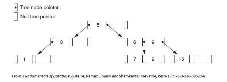
It's easy to see from this simple example that the values are maintained in sorted order. Further, each of the nodes in the tree has exactly three tree node pointers that can point to other nodes. That second fact makes this a tree of order 3. Fourth order trees will have four node pointers, fifth orders have five, and so on. There is no limit to the number allowed, but at some point there may be diminished returns because of the rearrangement that is necessary when we add or remove values. To take a simple example, consider if we wanted to add the value two or four into this tree. The operation is trivial, since the values can be put into existing empty spaces in the nodes of the tree, without having to do any re-ordering; simply insert the values. However, what about adding the value ten into the tree. Now we need to move the twelve over to make room for the ten in that node. Then, what about adding eleven? To do this, we need to move the six up beside the five, the seven takes six's place, eight moves over, nine moves down, ten moves up, and the eleven can now go next to the twelve. The reason this gets so complicated is we want to maintain, as much as possible, the depth of the tree across all the nodes. In this case, the tree has a depth of three, and by doing all those gyrations we maintain that depth. Any further additions, though, and we'll have to increase the depth by a level, and the whole thing gets re-arranged again! Indeed, we actually have the additional problem of trying to make sure the tree remains balanced.

Next: B-Trees

A B-Tree is an extension of the tree idea, to incorporate pointers to the data items that will need to be searched for in the database. In this case, as you can see, the values in the nodes have two parts instead of one, with the second part containing a pointer to the location on disk or in the file system that contains the data which would be searched for. Note that this is an index, the same as we saw above, and can basically take on any of the forms of index that were mentioned. Here is a handy diagram to show you what is meant:

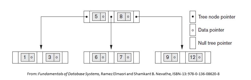
Inserting and deleting in this tree is the exact same process as in the normal search tree of order 3 as we saw previously. The only real difference here is the fact that the nodes have a data pointer as part of their definition.

Finally: B⁺-Trees

A B⁺-Tree takes the B-Tree one step further. It only allows the data pointers to be stored at the leaf nodes of the tree, meaning that the structure of leaf nodes is different from the structure of the internal nodes. Leaf nodes thus have an entry for every value of the search field, along with the data pointer to the record or block that contains the data or the record of interest. The records pointed to are most often key fields of some type, such as a primary key, or the records may end up being pointers to blocks of pointers, as we've seen above. Further, leaf nodes are linked to each other, with a special pointer at the end of the node that points to the next leaf node, making the structure of the leaves much like a singly-linked list structure. So, pointers in the internal nodes are tree pointers, while pointers in leaf nodes are data pointers except for the last [or P_next node] which points to the next leaf.

The following diagram shows the insertion sequence [directly from your text book] for inserting the values 8, 5, 1, 7, 3, 12, 9, and 6 into a B⁺-Tree. It is useful to follow the activity, to see just how this works.

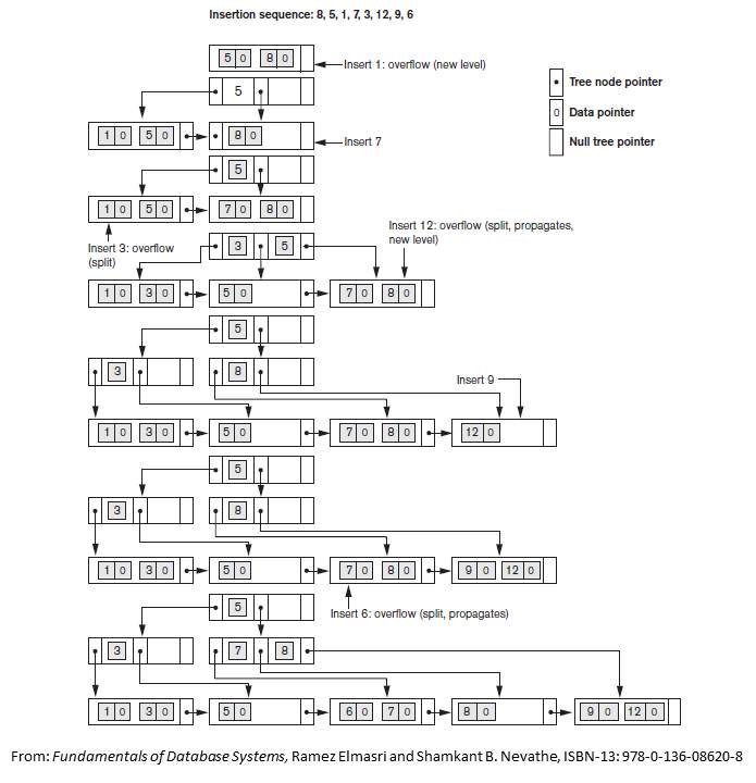
First, we observe that the root is the only node in the tree, so it is also a leaf node. As soon as more than one level is created, the tree is divided into internal nodes and leaf nodes. Notice that every key value must exist at the leaf level, because all data pointers are at the leaf level. However, only some values exist in internal nodes to guide the search. Notice also that every value appearing in an internal node also appears as the rightmost value in the leaf level of the subtree pointed at by the tree pointer to the left of the value.

When a leaf node is full and a new entry is inserted there, the node overflows and must be split. This split is made at roughly the 1/2 way point in the node, with the middle value being moved to the parent internal node, and a new pointer is created in the parent to point to the new node which ends up with the remaining values from the original leaf. If the parent is also full, it must be split as well, and so on and so on until everything balances out.

…and that's all I have to say about that, too…

Coming up…

Midterm Review Monday

MIDTERM EXAMINATION NEXT WEDNESDAY!!